 Scoop has an Ethical Paywall


Auckland Transport Blog: The Value of Time
The Value of Time
by Peter Nunns
July 3rd, 2013
http://transportblog.co.nz/2013/07/03/the-value-of-time/
Readers of this blog will be familiar with the notion of the benefit cost ratio (BCR), a figure that compares the forecasted benefits of a project with the financial cost of building it. It’s often used as a shorthand for the quality of a project: If the BCR is high (i.e. substantially above 1) it is seen as a good use of public money; if not, it can be criticised as a boondoggle.
Everyone plays this game. Opposition politicians often criticise motorway projects such as Puhoi-Wellsford and the Kapiti Expressway on the basis of BCRs that fall below 1, while the Minister of Transport has in the past expressed scepticism about the City Rail Link on the same grounds.
However, there is relatively little public discussion of the hows and whys of these seemingly consequential numbers. How, exactly, does one calculate a BCR?
The procedures for conducting an economic evaluation of a transport project are set out in excruciating detail in the Economic Evaluation Manual (EEM) published by the New Zealand Transport Agency. This manual defines the exact procedures that need to be followed when evaluating any transport project and specifies the values that should be used in the evaluation.
Read it at your leisure (or peril). Here’s the summary version.
The traditional method of estimating the economic benefits of a transport project involves three main steps.
First, you need to define the project carefully – that is, you need to figure out what you are planning to build, when you will build it, and the new service patterns that you’ll introduce as a result. Take, for example, the case of the Avondale-Southdown rail line, which is in the Auckland Plan but hasn’t been defined carefully enough to enable us to figure out what it will do. We can’t evaluate that until we know exactly what we’re building and when.
Second, you need to forecast the effects that the project will have on travel behaviour. Let’s stick with the example of Avondale-Southdown. In the short term, we might expect adding a new rail line to encourage some people to switch from buses or cars, thereby reducing congestion, and to encourage some people to take trips when they wouldn’t otherwise have travelled. In the longer term, it might change the patterns of population and employment location, by making it easier for people to live and work in certain places.
This forecasting is typically done by regional transport models, which estimate (on the basis of existing travel patterns and forecast changes to land use in a region) how people will get around in the future and how much time it will take them.
Third, you need to quantify the benefits of changes to travel behaviour. This is where the EEM comes in. It summarises the types of benefits that you should expect from transport projects, and defines values that allow you to monetise those benefits. Broadly speaking, the benefits considered in the EEM fall into four main categories:
• Reduced travel
time
• Reduced vehicle operating
costs
• Reductions in accidents and health
costs
• Reduced vehicle emissions.
(There are obviously a whole bunch of important things that are not assigned any value under this framework. We might, for example, want a transport system that provides us with a choice of multiple modes, or increases our resilience to shocks such as tectonic plate activity or sudden oil price increases. These benefits are often considered in other stages of the evaluation but not quantified.)
NZTA considers travel time savings to be the most consequential economic benefit. Forecast travel time savings make up the largest share of quantified benefits from most large transport projects in and around Auckland. This is based on the idea that the time we spent in transit could be spent more productively on other activities. If we weren’t stuck on congested road and PT networks, we would be working more, or doing things that we found at least as satisfying or remunerative as work. For many projects, the time savings on an individual trip might be small – but they can add up quite rapidly over large numbers of trips.
Take the case of the CRL. Removing the Britomart bottleneck is expected to increase capacity and hence frequency across the whole network. This will make it quicker for PT riders to get into the city centre. The effects are larger on the Western Line but still significant from the South and East, as this table released by Auckland Transport indicates:

Click for big version.
CRL time savings
In short, reductions in travel time are an important topic! So how, exactly, do we place a monetary value on them?
The answer is buried in the appendices to the EEM – Tables A4.1 and A4.2 to be exact. I’ve summarised some of the key features in two handy charts. Unfortunately, the figures themselves present some logical conundrums.
The first chart compares the value of time assigned to trips on urban arterial routes and in rural areas. Urban travel during the weekend is considered to be less valuable than weekday travel – which is fair enough, as most people work during the week. But – perplexingly – urban commuter travel is considered much less valuable than rural travel of any type.
In plain English, the EEM places a much higher value on the average JAFA’s time when s/he is on holiday in the Bay of Islands than commuting across the Harbour Bridge to get to work.

Is this logical? It’s hard to say, because the EEM contains no attribution or explanation for these figures. They are apparently derived from willingness-to-pay surveys , in which people are asked what value they place on their own time. But they don’t seem to bear any relation to differences in productivity, which is another important measure of the value of time.
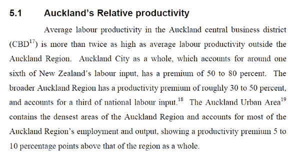
The econometric research suggests that urban areas in New Zealand, and in particular the Auckland city centre, have a large productivity premium over other areas. Take, for example, the findings of a 2008 paper by David Mare (“Labour productivity in Auckland firms” ). Based on this, one would expect Aucklander’s time to be counted as relatively more valuable, not less:
So far, so strange. Now look at the second chart, which compares the additional value of time assigned to commuter trips on different modes. The EEM places a much lower value on trips that aren’t taken in single-occupant cars. If you’re walking or cycling rather than driving, your time is worth $1 an hour less; if you’re taking the bus or train, it’s worth $3 an hour less.
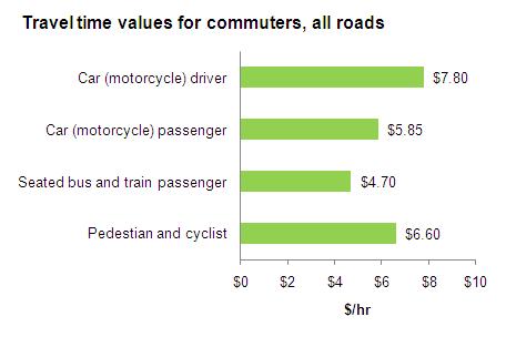
Once again, it’s impossible to say whether or not these values make any sense, because no source or attribution is provided. In theory, there might be some logic to these differences. For example, time spent in a bus might be less onerous as it enables one to multitask while travelling. And people might not object to time spent walking or cycling due to the health benefits. But counter-arguments could also be raised – many people enjoy driving cars and don’t mind spending a bit more time on the road.
What can be said is that the values of time defined in the EEM have consequences. They allow the transport outcomes from different projects to be quantified and compared with each other. Decisions about what to build and not to build are then based on those comparisons. So it’s tremendously important to know that we are evaluating projects using a method that undervalues the time of urban travellers relative to rural travellers, and undervalues the time of PT users, cyclists, and car-poolers relative to drivers.
Peter Nunns is an economist working in Auckland with an interest in transport past, present, and future.
 Binoy Kampmark: Catching Pegasus - Mercenary Spyware And The Liability Of The NSO Group
 Ramzy Baroud: The World Owes Palestine This Much - Please Stop Censoring Palestinian Voices
 Dee Ninis, The Conversation: Why Vanuatu Should Brace For Even More Aftershocks After This Week’s Deadly Quakes: A Seismologist Explains
 Martin LeFevre - Meditations: Meditation Without A Method
 Ramzy Baroud: Israel To Annex The West Bank – Why Now? And What Are The Likely Scenarios?
 Binoy Kampmark: The Strawman Of Antisemitism - Banning Protests Against Israel Down Under